Chapter 5
The OPAL Monte Carlo Environment

5.1  Monte Carlo Generation

In general, a Monte Carlo generator computes the cross-section for a physics process within certain boundary conditions, so called cuts, dictated by the experimental setup [58] [59]:

s = ó õ Pi f(fi)dfi

(5.1)

where the integration elements, df_i, are the multidimensional phase space variables and the integrand f(f_i) is the multi-differential cross-section, ¶s/¶f_i, composed of the matrix element squared and averaged of over spins, colors, and the phase space factors. The Monte Carlo method for computing s assumes that each integration element, df_i, can be re-expressed to span the unit hypercube where each element runs from 0 to 1. The volume of phase space is then given by

S = ó õ Pi dfi

(5.2)

To understand the Monte Carlo method, consider a set of random points f_i distributed uniformly over the phase space. The associated function values of f(f_i) are random numbers as well as the two important functionals,

R =  S N å j  Pi f(fij) W =  S2 N-1 å j  Pi f(fij)2-  1 N é ë å j  ( Pif(fij))2 ù û

(5.3)

where the product runs over the phase space variables, i = 1, 2, 3, ..., M, and the sum runs over the number of random points, j = 1, 2, 3, ..., N. The expectation values for these functionals are given by the integrals,

< R > = Pi si = s < W > = ó õ ( Pi f(fi) )2 dfi - é ë ó õ Pi ( f(fi) dfi ) ù û 2   = var(f)

(5.4)

The Monte Carlo method involves choosing the phase space variables f and calculating the phase space volume, S. A number, N, of random points f_i in phase space is picked and the values of f(f_i), R, and W are computed. The Monte Carlo estimate for s is given by R within 2/Ö(W/N) for a confidence level of 95% as implied by the Central Limit Theorem.

The Monte Carlo method holds independently of the dimension and shape of the phase space and allows for implementing any kind of cut by putting f(f_i) º 0 for f_i outside of the cuts. For the method to work, the only requirement is that one know S and that an algorithm to generate uniformly and independent values of f_i over the phase space exist. The error on the unweighted Monte Carlo method goes like 1/ÖN for large N, however various methods for weighting the Monte Carlos exist to produce events with smaller associated error. The most important of these methods is the method of importance sampling  [58] which consists of generating the variables f_i in such a way that there are more points where f(f_i) is larger. By making a transformation into a different integration variable, i.e. an approximate cross-section g(f_i), where

S` = ó õ i  g(fi)dfi

(5.5)

the formula for s can be written,

s = ó õ i   f(fi) g(fi) g(fi)dfi = ó õ i  w(fi)dfi¢

(5.6)

where

dfi¢ º g(fi)dfi  and  w(fi) º  f(fi) g(fi)

(5.7)

All Monte Carlo generators discussed in this thesis use importance sampling for many variables as well as random number generators with long period lengths (RNDM [58] with a period of 2²⁹ or RANMAR [60] with a period of 2¹⁴⁴).

5.2  Electroweak Effects in Monte Carlos

(1) Explicit Inclusion - The weak corrections are explicitly calculated based on the standard model Lagrangian and included in the program via the input parameters like MZ0, a(0), as(MZ02), GFermi, Mtop, MHiggs, etc.

(2) Implicit Inclusion - The weak corrections are not explicitly calculated but modelled using an approximate Born parameterization like


(s - MZ02)2 + GZ02 / MZ02 Þ (s - MZ02)2 + s2GZ02 / MZ02 sin2qw Þ sin2 qw   Þ sin2qw* a(0) » 1/137 Þ a(MZ02) » 1/128

(5.8)

The essential feature of QED corrections is the infrared divergencies in the real and virtual photon cross-sections which disappear only when they are combined. The root of the infrared divergencies can be seen to originate from fixed-order perturbation theory. The problem is resolved by dividing the cross-section into a soft and hard component through a cutoff parameter, k₀, and then going to infinite order in perturbation theory for the terms with highest power of ln(k₀). The total cross-section for an arbitrary number of soft photons can be directly related to the ``bare'' cross-section due to the exponentiation of the k₀-parameter. This exponentiation can be implemented in Monte Carlo programs in three distinct ways:

(1) Ad-hoc Exponentiation: [61] The total energy loss due to brehmsstrahlung is used to modify a first-order Monte Carlo program to take into account the additional factor k^b in


¶s ¶k » s0 ×  b k ×kb

(5.9)

Here, the total energy loss due to brehsstrahlung is obtained from the derivative of s^{S₁S₂S₃...} with respect to k₀.

(2) Structure Functions [62]: The application of structure functions to the QED allows the total cross-section to be described as a convolution of the lowest-order cross-section at reduced energy and another containing the photon emission according to


s(s) = ó õ 1 0  dx F(s,x)s0(xs)

(5.10)

Here, F(s,x) denotes the structure function and xs = s^¢ is the remaining effective energy, which can take all values between 1 and s. The exponentiation is now implemented in the definition of F(s,x).

(3) YFS Exponentiation: The application of methods by Yennie, Frautschi, Suura (YFS) [63] to construct realistic multiple photon Monte Carlo programs for e⁺e^- ® f[`(f)] + n(g). The amplitude of the contribution from n virtual photon loops in the initial state, summed over n has the form


M = eaB ¥ å n=0  mn

(5.11)

This formulation leads to a rigorous calculation of the infrared singularity to all orders of a on an event-by-event basis.

Regardless of the scheme for exponentiation used, the Monte Carlo method consists of determining the soft photon spectrum (bremsstrahlung) of the form

f(x) º ( bln(k0) + df ) d(k0) +  b x q(x-k0)

(5.12)

where x is the photon energy, k₀ is the soft and hard photon cutoff, and d(x) is the soft and virtual photon contributions. The total energy loss due to 0-g, 1-g, 2-g, 3-g, ... soft photons is given by the spectrum function,

P(x) º d(x) + ó õ x 0  dx1 f(x1) d(x1 - x) +  1 2! ó õ x 0  ó õ x 0  dx1 dx2 f(x1) f(x2) d(x1 + x2 - x) +  1 3! ó õ x 0  ó õ x 0  ó õ x 0  dx1 dx2 dx3 f(x1) f(x2) f(x3) d(x1 + x2 + x3 - x) + . . .

(5.13)

This can be re-expressed by integrating exactly those parts of f(x_i) that go with d(x_i) to give

P(x) º ebln(k0)+df Q(x)

(5.14)

where

Q(x) º d(x) + b ó õ x k0  dx1  1 x1 d(x1 - x) +  b2 2! ó õ x k0  ó õ x k0  dx1 dx2  1 x1 x2 d(x1 + x2 - x) +  b3 3! ó õ x k0  ó õ x k0  ó õ x k0  dx1 dx2 dx3  1 x1 x2 x3 d(x1 + x2 + x3 - x) + . . .

»  b x ebln(x/k0) ×  e-bC G(1+b)

(5.15)

By picking terms of Q(x) which correspond to real photon multiplicities, the appropriate matrix elements can be generated. This element is multiplied by the overall factor e^{bln(k₀)+d_f} which is compensated by the fact that as k₀ ® 0, the factor ln(x/k₀) in Q(x) increases. The result is that the higher-order terms become numerically more important with the additional photons becoming softer.

5.3  Electroweak Monte Carlo Generators

5.3.1  The NNG04 Monte Carlo

The NNG04 Monte Carlo program [64] was written by M. Mana and M. Martinez in collaboration with F. Berends and G.J.H. Burgers to generate the cross-section and simulate events for the radiative signal, e⁺e^-® n[`(n)]g(g). The total cross-section for the e<sup>+</sup>e<sup>-</sup>® n[`(n)]g signal at Ös » M_Z⁰is determined by summing the contributions from processes like the Z⁰ self energy (+15%), the soft photon and QED corrections (-48%), and the double hard brehmsstrahlung (+37%). The program uses exponentiation of the initial state soft photon together with a ``star-scheme'' treatment of the weak corrections.

The program models the Feynman diagrams shown in Figure 2.1 and uses the input parameters shown in Table 5.1 [64]. The program generates events for a maximum number of trials, NT, with a specific number of integration points, NP. The program performs calculations of the single photon final state, e⁺e^-® n[`(n)]g, and the double hard bremsstrahlung process, e<sup>+</sup>e<sup>-</sup>® n[`(n)]g(g), quoting a final cross-section, the soft plus virtual QED corrections and the Z⁰ self-energy correction. The program has been studied against other generators including KORALZ [65] and MOE [66] and has demonstrated agreement to within 2% [67] for events with one photon with E_g > 0.4 GeV and q_g > 10 deg.

5.3.2  The TEEGG Monte Carlo

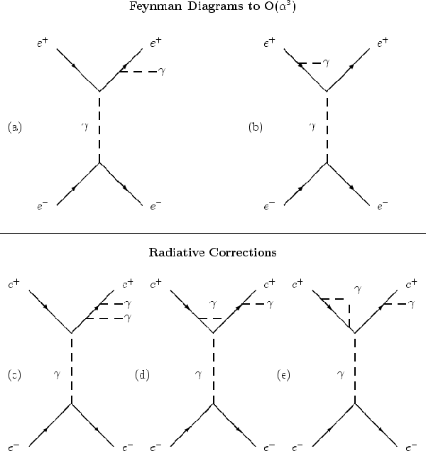
The TEEGG Monte Carlo program [68] was written by D. A. Karlen to simulate the radiative Bhabha process, e⁺e^-® e⁺e^-g(g), for low Q² configurations where the electron and/or positron scatter at small angles. The dominant diagram is the t-channel amplitude which require the evaluation of QED radiative correction to O(a⁴), while neglecting the contribution from the Z⁰ as shown in Figure 5.1. The lowest-order cross-section calculation is based on the wide angle scattering algorithm of Berends and Kleiss [69] with additional mass terms. The O(a⁴) QED radiative corrections are evaluated by the equivalent photon approximation where only the t-channel amplitudes and the radiative corrections to the sub-process of Compton scattering are included. The infrared divergence is also incorporated with a soft photon cutoff parameter, k₀, defined in the rest frame of the colliding electron and photon.

The Monte Carlo requires the input parameters as shown in Table 5.2  [68] and reproduces reliable results within the range of validity for the O(a⁴) QED radiative corrections. The program has been tested with data from the Mark II detector for configurations where both an electron and photon scatter at large angles. The results indicate that the data and the calculations agree within the experimental uncertainty of 2% for events with one photon with E_g > 0.5 GeV and q_g > 45 deg [69].

5.3.3  The RADCOR Monte Carlo

The RADCOR Monte Carlo program [72] was written by F.A. Berends and R. Kleiss to simulate two and three photon final states for the process, e⁺e^-® gg(g). Unlike m⁺m^- pair production and Bhabha scattering which are influenced by the weak interaction and polarization effects at higher energies, the e⁺e^-® gg(g) process is completely QED. The RADCOR program models the process by incorporating the infrared divergence with a soft photon cutoff parameter, k₀, and differentiating two final states: i)the soft photon with no bremsstrahlung, ii)the hard photon which generates bremsstrahlung above the k₀ cutoff parameter.

The lowest-order cross-section is used to determine the weights associated with the generated final state photons. Virtual corrections are determined for each weighted event and used to determine the total cross-section contribution for each event to O(a³). The Monte Carlo uses the input parameters shown in Table 5.3  [72] and has been studied with large samples of events demonstrating good agreement with expected results to within 1% for events with one photon with E_g > 0.4 GeV and q_g > 10 deg  [72].

5.3.4  The TWOGEN Monte Carlo

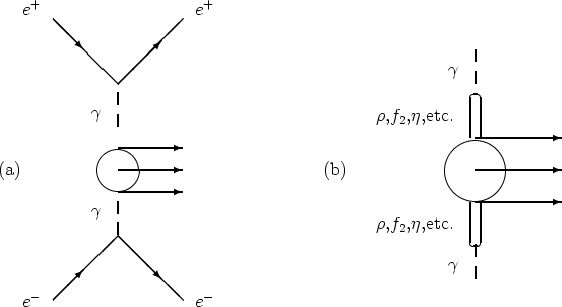
The TWOGEN (TWOGEN11) Monte Carlo [73] was written by W. Langeveld to produce both pairs and multihadronic states via the two-photon process for e⁺e^-® e⁺e^-X. The program was later modified by A. Buijs and G. J. VanDalen to produce resonance states including X® f₂,p⁰,h,h¢ which eventually decays into final state photons. The program is one of two programs used in the analysis presented in this thesis to study the specific generation of events via the two-photon process. TWOGEN generates resonance events in three distinct steps:

(1) Events are generated according to the exact transverse-transverse luminosity function given by G. Bonneau, M. Gourdin and F. Martin [74].

(2) A resonance is produced from the available states, i.e. X® f₂,p⁰,h,h¢, according to weighting through the vector dominance model form factor (r).

(3) The resonance decays according to the LUND Monte Carlo and tracks are transformed from the gg center-of-mass as shown in Figure 5.2.

The program has been used by various groups and demonstrates consistent results for the phase space considered, i.e. within 5% for events with one photon within q_g > 20 deg. and E_g > 0.5 GeV [75]. The Monte Carlo makes use of the input parameters shown in Table  5.4 [73].

5.3.5  The VERMAS Monte Carlo

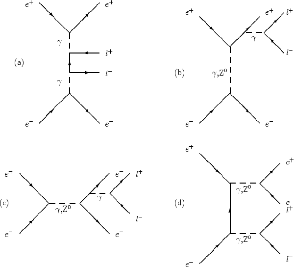
The VERMAS (VERMAS10) Monte Carlo program [76] was written by G.P.Lepage, J. Smith and J.A.M. Vermaseren and later modified by G. J. VanDalen. It is the second of two programs (see Section 5.3.4 for TWOGEN) used in the analysis presented in this thesis to study the specific generation of events via the two-photon process. VERMAS generates e⁺e^-® f[`(f)] to order O(a⁴) through QED matrix elements. Here f can be e^-, m^-, t^-, u, d, s, c, or b. The program uses an exact seven-dimensional numerical calculation of the total cross-section with Mandelstam-type variables for the Feynman diagrams shown in Figure 5.3. The Monte Carlo requires the input parameters shown in Table 5.5  [76]. Calculations of the program have been checked against the double-equivalent-photon approximation (DEPA) and has demonstrated agreement to within 1% of these results [77].

5.3.6  The KORALZ Monte Carlo

The KORALZ (KORALZ38) program [78] was written by S. Jadach, B.F.L. Ward, and Z. Was to generate fermion pairs, e⁺e^-® f[`(f)], where f can be e^-, m^-, t^-, u, d, s, c, or b. The program includes the complete electroweak radiative corrections to O(a), initial and final state QED bremsstrahlung, t-decay modes and polarization effects, and beam polarization effects. The program does not include QED initial-final state bremsstrahlung interference for multiple QED hard bremsstrahlung in the initial state and multi-pion t-decay modes. KORALZ generates events in three distinct steps:

(1) Fermion pairs including QED bremsstrahlung, spin effects and the electroweak corrections are produced.

(2) The TAUOLA library is used to simulate t-decays into seven exclusive channels, i.e. [`(n)]en, [`(n)]mn, [`(n)]p, [`(n)]r, [`(n)]a<sub>1</sub>, [`(n)]K, and [`(n)] K^-, and into multi-pion decay channels along with leading-log QED radiative corrections.

(3) The O(a) electroweak radiative corrections from the standard model are combined with gluonic (hadronic) effects.

5.3.7  The BABAMC Monte Carlo

The BABAMC (RADBAB20) program [79] was written by R. Kleiss, F.A. Berends and W. Hollik to generate Bhabha scattering events, e⁺e^-® e⁺e^-g, for use in the determination of luminosity. The program includes the complete electroweak and vacuum polarization corrections due to fermions from e⁺e^- to O(a). The program uses a multi-channel approach to include explicit corrections to the cross-section in five distinct channels:

(1) Initial-state radiation in the s-channel, with photon exchange.

(2) Final-state radiation in the s-channel, with both photon and Z⁰ exchange.

(3) Initial-state radiation in the s-channel, with Z⁰ exchange.

(4) Bremsstrahlung in the t-channel, with photon exchange.

(5) A Born term with weak corrections and QED corrections from virtual photons and soft bremsstrahlung.

5.4  The OPAL Detector Simulation

1. At initialization time the geometrical description of the detector, the materials and tracking parameters for each volume are defined.
   
2. Primary kinematics for each event are generated.
   
3. As each particle traverses a sensitive detector, ``hits'' are stored which contain the necessary information to allow the subsequent simulation of the detector response. In addition, GEANT decides whether to stop the tracking of certain particles based on the energy or lifetime of the particle.
   
4. At the end of each event the hits are used to simulate the data which the detector would have produced for subsequent reconstruction or analysis.

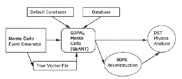
Using the GEANT package, the GOPAL code simulates the full OPAL detector consisting of 15 subdetectors and all the passive elements such as the magnet coil, the beam pipe, and pressure vessel, with a total of more than 49 different materials and 68,413 volumes, nested up to 12 deep. The constants associated with the various subdetector elements are also read in and recorded for the event just before the first event for use in the digitization. The program then obtains the kinematics for the primary event in one of two ways: first, the run generator inside GOPAL provides the necessary KIUSER interface for the event, or second, a standard ``four-vector'' file is accessed which has been previously produced by an event generator in stand-alone mode. The GOPAL representation of the generated events, the TREE Bank, is a special structure consisting of 22 words per particle containing: i) the four-momentum, ii) the mass, charge and PDG particle ID, iii) the spatial coordinates of the particle trajectory, iv) the pointers to parent and daughters, and v) the start and end flags for tracking.

When a particle traverses the sensitive region of a detector, the raw signals of the detector are generated. The tracking of the particle is completed by storing the position and momentum of each charged particle at tracking time. The interaction of each particle is simulated step-by-step along its path. Such interactions with the material include energy loss, multiple scattering, bremsstrahlung, decay in flight and nuclear interactions. The EGS [84] program is used to simulate electromagnetic interactions in the dense materials, while the GHEISHA Monte Carlo [85] handles the nuclear interactions. In addition, the short-lived particles such as K_s, p₀ and L are allowed to decay in the simulation leaving secondary vertex information. The tracking for all particles, e.g. primary, secondary, etc., is completed together and the response to each track segment is computed using a parameterization technique before digitization.

During the digitization, the HITS information is collected and the response of the detector is determined. Except for the lead glass electromagnetic calorimeter, all subdetectors require an elaborate simulation response treatment. This treatment fills the simulated raw data structure for each subdetector using special digitization code tuned for each detector. The data structure at the end of GOPAL looks exactly like that emerging from the OPAL detector including simulation from the OPAL trigger. The data structure from GOPAL consisting of a constant record and events can be analysed by the Reconstruction program of OPAL (ROPE) to produce a data summary tape (DST) for analysis or histograms of NTUPLES. The ROPE processing can either occur directly in GOPAL for increased efficiency and time saving or can occur separately from the GOPAL processing in a stand-alone mode. Once the ROPE data structure (banks) are generated, the events can be displayed in the off-line environment using the OPAL event display program, GROPE. Note that the GROPE processor allows reconstructions of all OPAL events whether ``real'' data or simulated Monte Carlo as discussed in Section 4.6. The whole simulation system is diagrammatically displayed in Figure 5.4 [86].

Performance of the Detector Simulation

The GOPAL Monte Carlo simulation code is capable of operating in stand-alone mode to help in the reconstruction and analysis code development as well as debugging or in parallel mode to increase the speed of simulation. The time taken by the GOPAL simulation code to simulate a typical multihadronic event, e⁺e^-® Z⁰® q[`(q)]® hadrons, is rather long as shown in Table 5.8 [86]. Although the reconstruction time is dominated by the central tracking, the simulation time is dominated by the shower development in the lead glass, compared to about 10% in the central tracking chambers. A ``bootstrap'' option is available to perform the shower simulation for any electron or photon below some cutoff, e.g. 500 MeV, by choosing a previously generated shower at random from a library. This speeds up the lead glass shower simulation by a factor of three, although the fitted data is not quite as good as the full shower development. Tracking routines speed up simulation in the forward detector by allowing four bremsstrahlung photons to be generated during one tracking and skipping intermediate tracking. However, the bootstrap method suffers from the following difficulties: i) the poor agreement of the bootstrap results with the data when compared to the full shower development, ii) the need for updating the parametrizations for each new version of GEANT, and iii) the unresolved problems with leakage for the electromagnetic component of hadronic showers.

However, the most effective fast simulation is obtained by using a simplified form of the GEANT geometry and tracking termed the ``SMEAR'' mode. This mode employs simplified geometry in the central detector, the calorimeter, and the muon chambers with tracking cutoffs, tuned parameters, and a quick smearing procedure of the track parameters. This mode of simulation has the notable draw back of poor agreement for multi-particle and overlapping electromagnetic showers, but increases speed on the average by a factor of 100 with acceptable results.

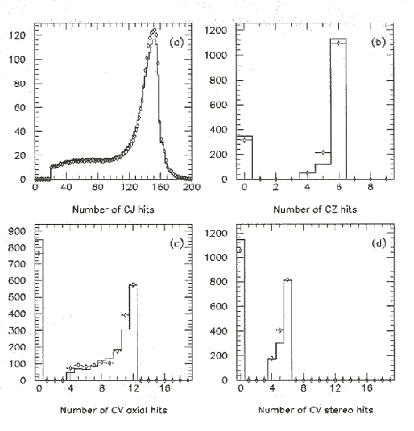
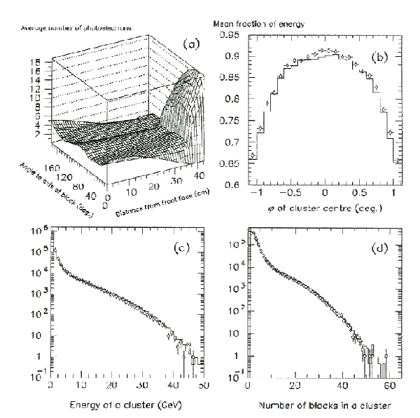
In the simulation of the central tracking chambers, each wire signal is generated from the energy loss of the track near the wire. The energy loss is calculated based on the dE/dx versus momentum curve determined from the data. A comparison of the data from the multihadron events with the GOPAL Monte Carlo simulation shown in Figure 5.5 [86] indicates good agreement. In the simulation of the electromagnetic calorimeter, the shower process is modelled using the ``Bootstrap Method'' [87]. For relatively high particle energies, the energies deposited are calculated using the EGS program. For particle energies of less than 100 MeV, the energies deposited are determined from a table search of pre-calculated shower energies corresponding to various incident energies of particles and gives a fast calculation of the shower energy. In either case, the calculated shower energy is finally translated into the pulse heights of photomultipliers attached to the each lead glass counter. The agreement between the data and GOPAL Monte Carlo simulation for different parameters of the electromagnetic energy is seen to be good as shown in Figure 5.6 [86].